Cluster Analysis

MDANCE provides a pipeline to screen the optimal number of clusters for a given dataset.

The pwd of this script is $PATH/MDANCE/examples.

To begin with, let’s first import the modules we will use:

import matplotlib.pyplot as plt
import numpy as np

scores_csvs is the list of screening csv that were outputted from screen_nani.py. The output of this notebook will also be the same directory as the input csvs.

scores_csvs = ['../scripts/nani/outputs/10comp_sim_summary.csv']

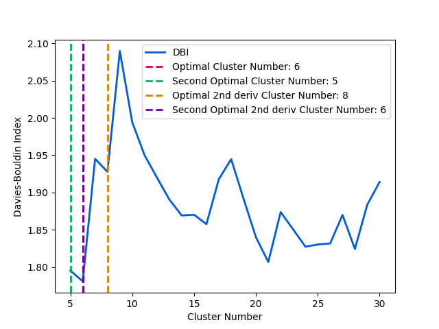
The function below will plot the Davies-Bouldin index and the optimal number of clusters.

• The optimal number of clusters is determined by the minimum Davies-Bouldin index or the minimum of the second derivative of the Davies-Bouldin index.

• Potential Errors

  • Please remember to remove the row with None,None in the screening csv if there is an error.

def plot_scores(scores_csv):
    """Plot the Davies-Bouldin index and the optimal number of clusters.

    Parameters
    ----------
    scores_csv : str
        The path to the csv file that contains the screening

    Returns
    -------
    file
        A png file that contains the plot of the Davies-Bouldin index and the optimal number of clusters
    """
    base_name = scores_csv.split('\\')[-1].split('.csv')[0]
    n_clus, db = np.loadtxt(scores_csv, unpack=True, delimiter=',', usecols=(0, 3))

    # Plot the Davies-Bouldin index and the optimal number of clusters
    all_indices = np.argsort(db)
    min_db_index = all_indices[0]
    min_db = n_clus[min_db_index]
    all_indices = np.delete(all_indices, 0)
    second_min_index = all_indices[0]
    second_min_db = n_clus[second_min_index]

    fig, ax = plt.subplots()
    ax.plot(n_clus, db, color='#005cde', label='DBI', linewidth=2)
    ax.set_xlabel('Cluster Number')
    ax.set_ylabel('Davies-Bouldin Index')
    ax.axvline(x=min_db, color='#de005c', linestyle='--', label=f'Optimal Cluster Number: {int(min_db)}', linewidth=2)
    ax.axvline(x=second_min_db, color='#00ab64', linestyle='--', label=f'Second Optimal Cluster Number: {int(second_min_db)}', linewidth=2)

    # Calculate the second derivative (before + after - 2*current)
    arr = db
    x = n_clus[1:-1]
    result = []
    for start_index, n_clusters in zip(range(1, len(arr) - 1), x):
        temp = arr[start_index + 1] + arr[start_index - 1] - (2 * arr[start_index])
        if arr[start_index] <= arr[start_index - 1] and arr[start_index] <= arr[start_index + 1]:
            result.append((n_clusters, temp))
    result = np.array(result)
    if len(result) == 0:
        print('No maxima found')
    elif len(result) >= 1:
        sorted_indices = np.argsort(result[:, 1])[::-1]
        sorted_result = result[sorted_indices]
        min_x = sorted_result[0][0]
        ax.axvline(x=min_x, color='#de8200', linestyle='--', label=f'Optimal 2nd deriv Cluster Number: {int(min_x)}', linewidth=2)
        if len(sorted_result) >= 2:
            sec_min_x = sorted_result[1][0]
            ax.axvline(x=sec_min_x, color='#6400ab', linestyle='--', label=f'Second Optimal 2nd deriv Cluster Number: {int(sec_min_x)}', linewidth=2)

    ax.legend(fontsize=10)
    plt.show()

if __name__ == '__main__':
    for scores_csv in scores_csvs:
        plot_scores(scores_csv)